Introduction
The global supply chain is responsible for approximately 24% of worldwide CO2 emissions. As organizations face mounting pressure to hit Net Zero targets, traditional logistics planning—often siloed by mode (truck, rail, sea, air)—is no longer sufficient. Enter the Multimodal Optimal Transport (MOT) simulator: a sophisticated computational framework designed to minimize carbon intensity while maximizing operational efficiency. By leveraging mathematical optimization and real-time data, these simulators allow climate tech leaders to visualize, stress-test, and refine complex supply chains before a single vehicle leaves the loading dock.
In this article, we explore how MOT simulators function, how they can be deployed to reduce Scope 3 emissions, and the strategic advantages they offer in a decarbonizing economy. For a broader perspective on how technology is reshaping business efficiency, see our guide on business innovation strategies.
Key Concepts
At its core, a Multimodal Optimal Transport simulator solves a version of the “Kantorovich problem” applied to logistics. It treats the movement of goods as a flow distribution problem across a network of heterogeneous transport modes. Unlike standard route planners, an MOT simulator weighs the cost of carbon alongside the cost of capital and time.
Key pillars of MOT simulation:
- Modal Shift Analysis: Calculating the precise tipping point where transitioning from road freight to rail or inland waterway reduces emissions without violating service-level agreements (SLAs).
- Last-Mile Optimization: Integrating electric vehicle (EV) fleet constraints into the broader multimodal journey to ensure seamless handoffs.
- Stochastic Modeling: Accounting for real-world variables like port congestion, extreme weather events, and energy price volatility.
By simulating these variables, companies can transform their logistics from a reactive cost center into a proactive climate solution. For those interested in the foundational math behind these systems, the National Renewable Energy Laboratory (NREL) offers extensive research on freight mobility and energy efficiency.
Step-by-Step Guide: Implementing an MOT Simulator
Transitioning to an MOT-driven model requires a structured approach to data integration and algorithmic calibration.
- Data Aggregation and Normalization: Collect historical logistics data, including SKU-level weight, delivery windows, and existing mode-specific emission factors. Ensure data from disparate ERP and TMS systems is normalized.
- Defining the Objective Function: Clearly define your KPIs. Is the goal absolute carbon reduction, or is it a balance of cost-per-unit and carbon-per-unit? An MOT simulator is only as good as the weights you assign to these variables.
- Network Mapping: Create a digital twin of your supply chain network. Map every node (warehouses, ports, transshipment hubs) and every possible edge (transportation lanes) with their respective emission intensities.
- Simulation and Stress Testing: Run “what-if” scenarios. For example, simulate the impact of a 20% increase in fuel costs or a disruption in a major sea lane. Observe how the simulator re-routes cargo to maintain efficiency.
- Execution and Feedback Loop: Integrate the simulator’s output into your operational workflow. Use the results to adjust procurement strategies and logistics partnerships.
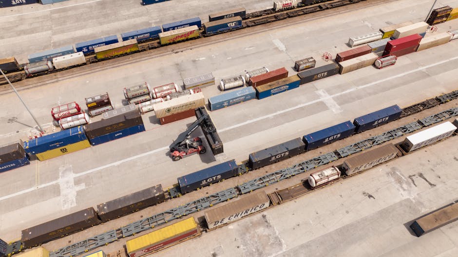
Examples and Case Studies
The practical application of MOT simulators is already changing how global giants operate. Consider a multinational consumer goods company shipping high-volume household products from Southeast Asia to Europe.
Traditional planning would likely rely on a mix of air freight for speed and ocean freight for cost. An MOT simulator, however, might identify a ‘slow-steaming’ ocean route combined with an electrified rail bridge through Central Asia. This approach maintains the delivery window while cutting the carbon footprint by up to 40% compared to traditional air-sea combinations.
Another real-world application involves urban last-mile delivery. By using MOT simulators to coordinate the arrival of heavy long-haul trucks at peripheral micro-hubs, companies can trigger “load-balancing” for e-bike or EV van fleets. This prevents the “idle-time” emissions that plague traditional distribution centers. For further reading on public policy and infrastructure support, visit the U.S. Department of Transportation’s resource hub on sustainable infrastructure.
Common Mistakes
Even with advanced software, implementation often fails due to common oversights:
- Ignoring Data Silos: Using incomplete data from one department (e.g., procurement) while ignoring another (e.g., fleet management) results in a “local optimum” that fails to produce global supply chain improvements.
- Over-reliance on Static Models: Logistics is dynamic. Failing to incorporate real-time weather, traffic, and energy cost feeds makes your simulation obsolete the moment it is run.
- Neglecting Human Factor Constraints: A simulator might suggest a perfectly efficient route that violates driver rest-time regulations or union agreements. Always include legal and labor constraints in your variables.
- Lack of Stakeholder Alignment: If the logistics team is incentivized solely on cost reduction, they will ignore the carbon-saving suggestions of the simulator unless sustainability is integrated into the bonus structure.
Advanced Tips
To extract maximum value from your MOT simulator, move beyond simple routing and into predictive intelligence.
Predictive Energy Hedging: Use the simulator to plan shipments around peak renewable energy generation times on the grid. If your fleet is electrified, aligning your charging schedule with grid availability is a massive win for sustainability.
Intermodal Synchronization: The most significant efficiency gains are found at the “hand-offs” between modes. Use your simulator to optimize buffer stocks at transshipment points. If a train is delayed, the simulator should automatically adjust the “last-mile” dispatch time to prevent empty-running vehicles at the destination terminal.
For those interested in the broader economic implications of these technologies, exploring The International Energy Agency (IEA) reports on transport energy consumption is highly recommended to understand how macro-trends influence your micro-logistics decisions.
Conclusion
Multimodal Optimal Transport simulators are no longer optional for climate-conscious enterprises; they are a fundamental requirement for operational resilience. By mathematically optimizing the interplay between cost, speed, and carbon, businesses can decouple their growth from their environmental impact. The shift requires moving away from static spreadsheets and toward dynamic, data-driven simulation environments.
Start small: identify a single high-impact lane in your supply chain, model it, and prove the efficacy of the multimodal approach. As the technology matures, these simulators will become the “brain” of the logistics network, guiding every decision toward a more sustainable and efficient future. For more insights on scaling these high-level strategies within your own organization, continue your journey at The Boss Mind.